Literature analysis
Here I discuss the various literature packages in R and show a use case on a topic I study. Available packages;
- bibliometrix: has a variety of functions returning most useful metrics you could want
- scholar: useful to evaluate journals and scholars (here I use it to retrieve impact factors of journals)
- pubmed.mineR: allows to query PubMed in multiple ways (great option if your query results is very high, but it’s slow and you won’t get citation counts and pubtator data)
- wosr: If you have an API username and password, this might be the best option to query a large amount of papers
- other packages: pubmedR, RISmed and RISmed
After spending some time exploring the different options, I found that MeSH terms were often missing, and Keywords or Keywords plus were not very informative. I ended up finding the results from pubtator. This is a NCBI Deep learning algorithm that identified and categorised 5 class of words in publications (Genes, Diseases, Mutations, Chemicals, Species) from the PMID. For use cases where you have a large number of results, I provide a script at the end of the document.
Aims:
- Determin the Keywords associated to the 14q32 locus evolution in time
- Determin journals yielding most citations on the subject
The following data was retreived from Web of science database with the following search therms: TOPIC: ((14q32) OR (DLK1-DIO3)) AND TOPIC: (heart OR cardi) The results were exported as plain text files.
pacman::p_load(bibliometrix,
               pubmed.mineR,
               rio,
               ttutils,
               tidyverse,
               ggplot2,
               ggrepel,
               scholar,
               reshape2)
Overview of the results
f <- c("data_litterature_14q32/14q32_OR_DLK1-DIO3_AND_heartORcardio.txt")
M <- convert2df(file = f, dbsource = "wos", format = "plaintext")
##
## Converting your wos collection into a bibliographic dataframe
##
## Done!
##
##
## Generating affiliation field tag AU_UN from C1: Done!results <- biblioAnalysis(M, sep = ";")
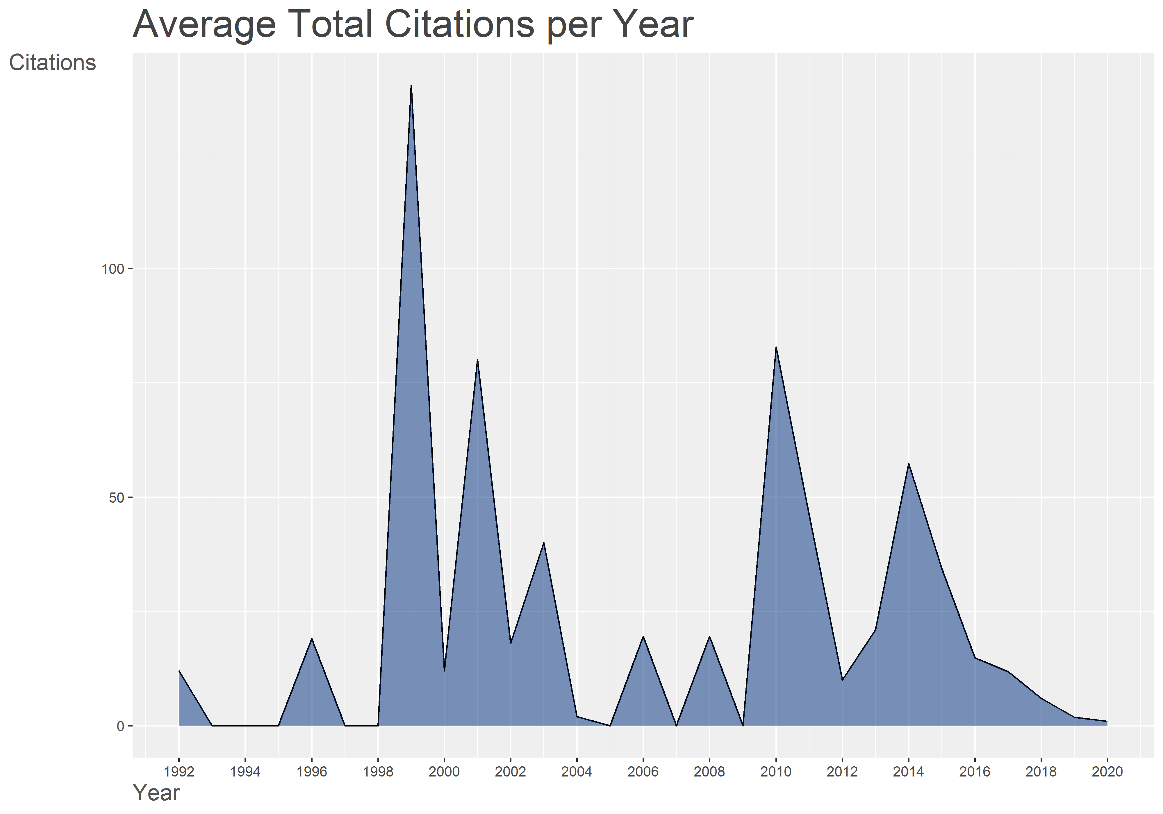
plot(x = results, k = 10, pause = FALSE)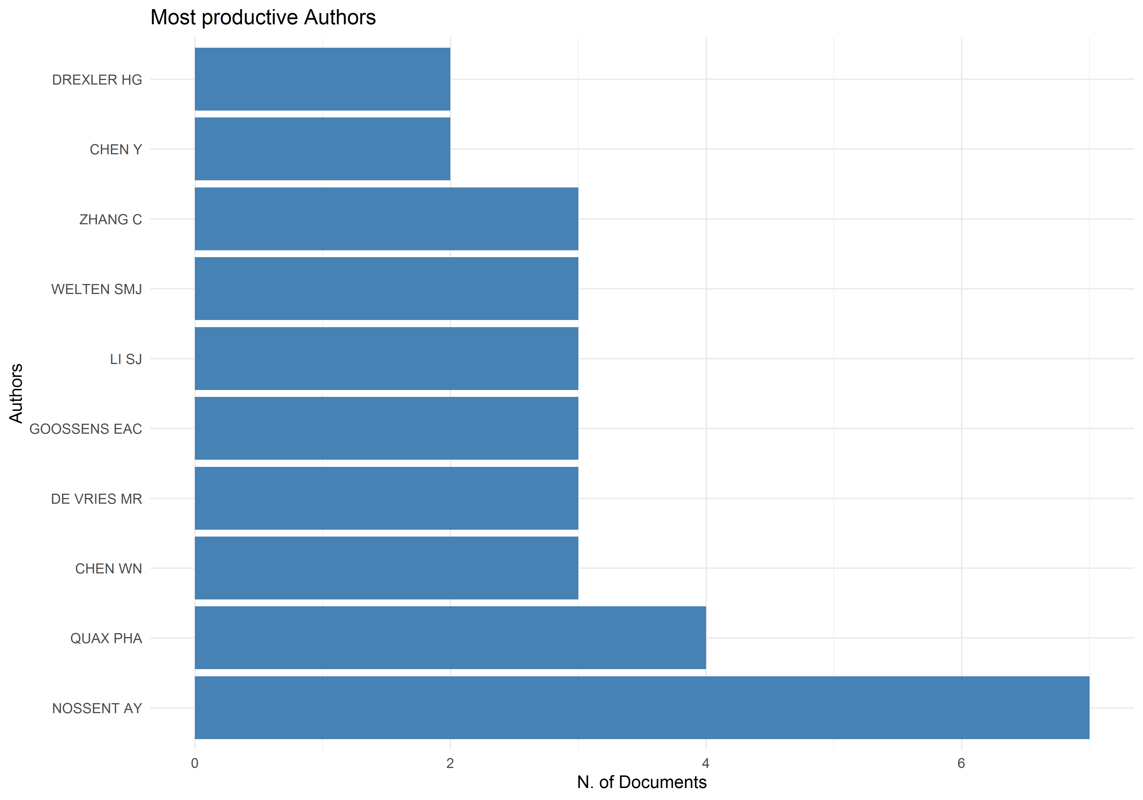
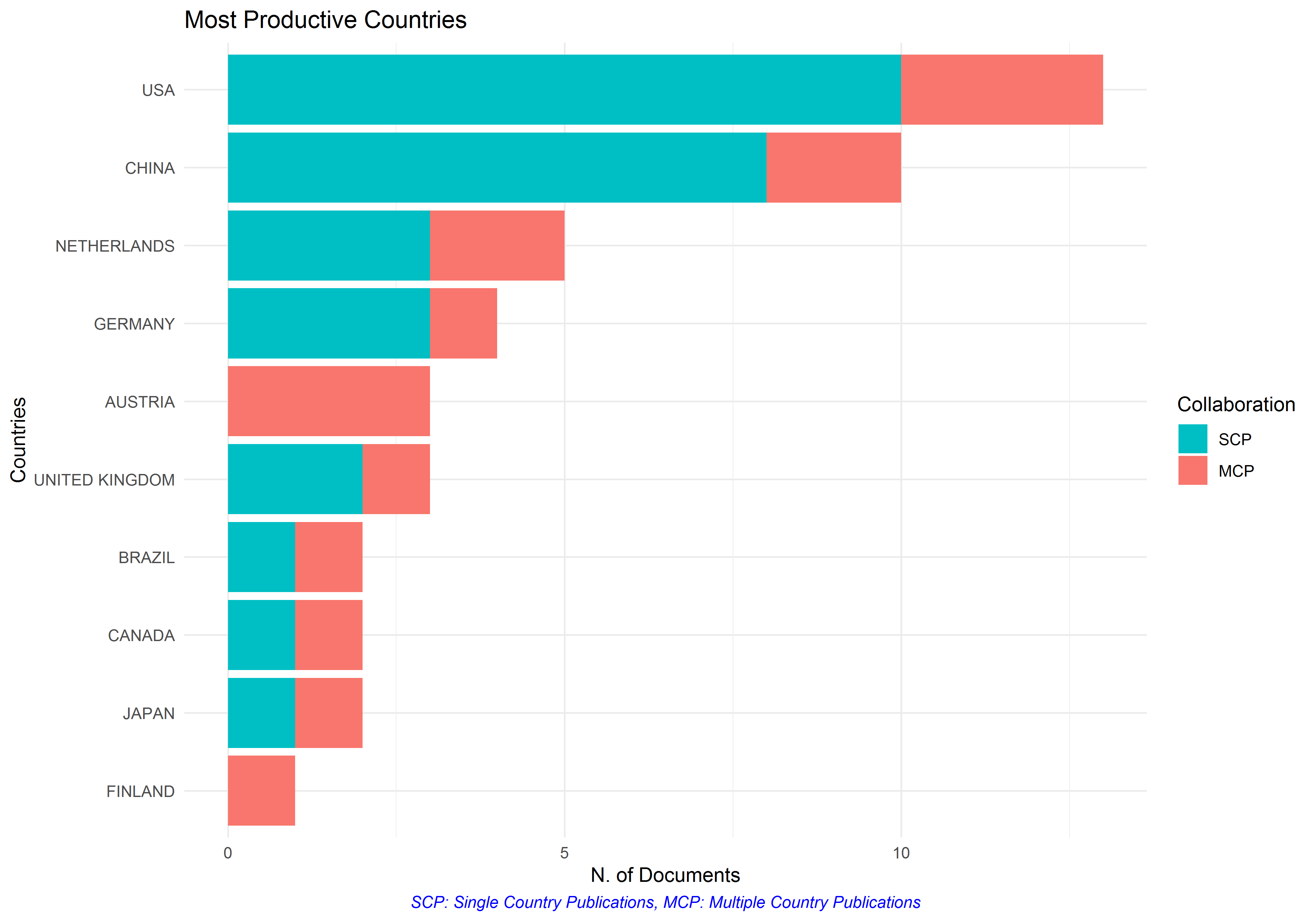
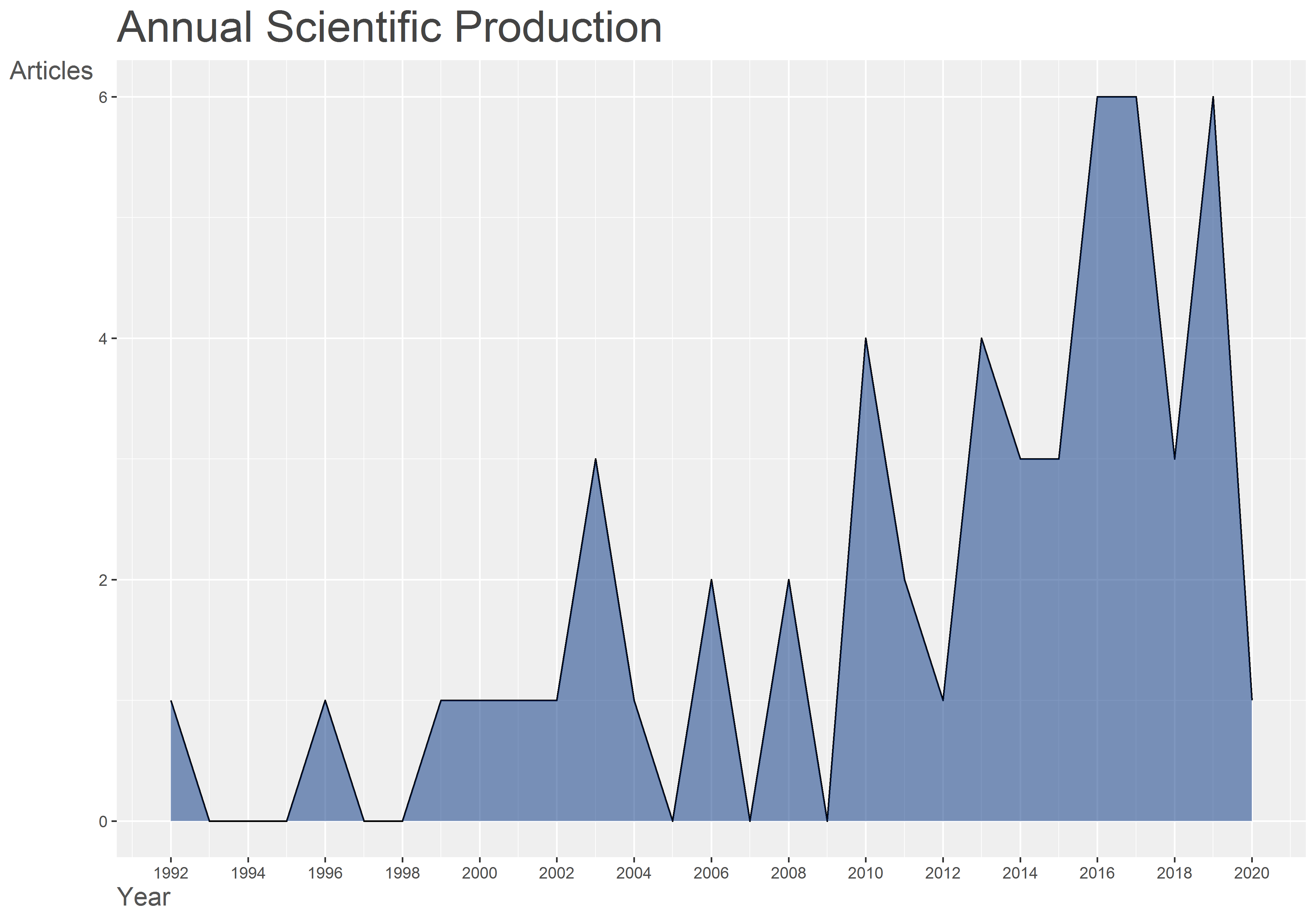
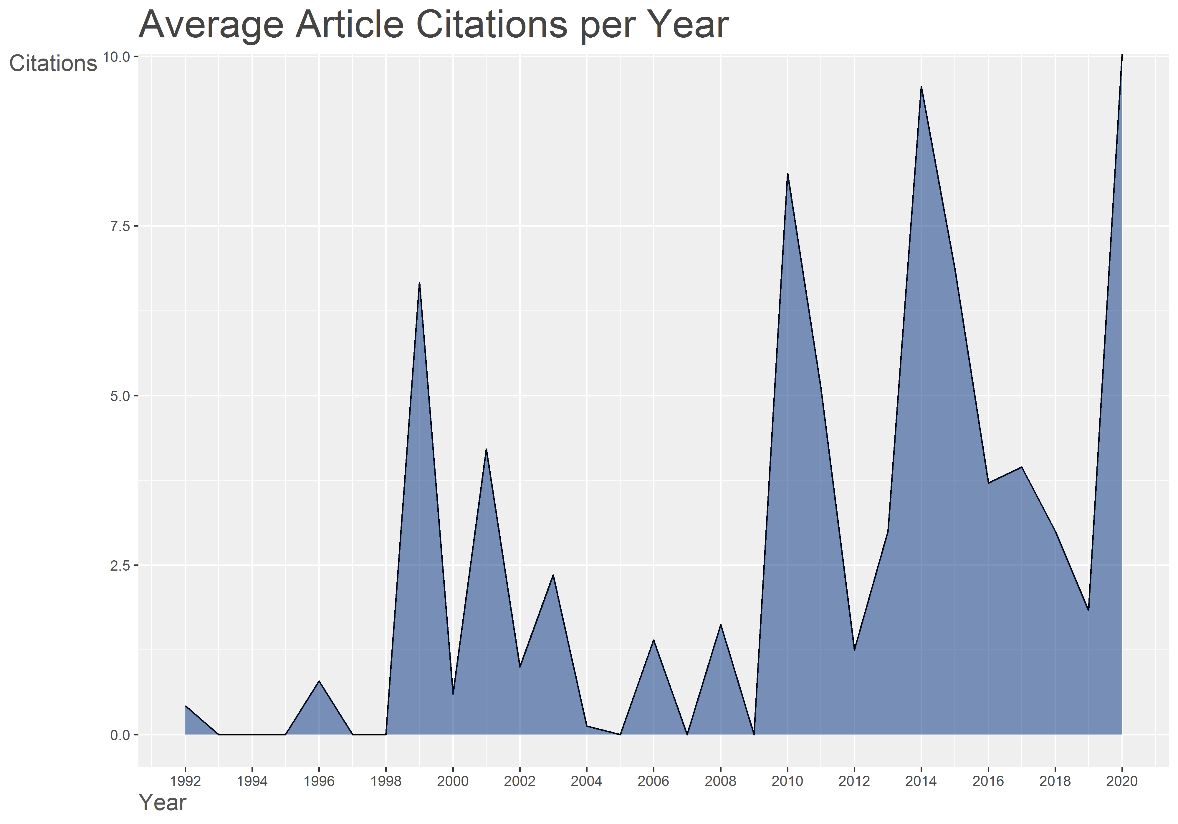
Co-occurence of Author Keywords
# Create keyword co-occurrences network
NetMatrix <- biblioNetwork(M, analysis = "co-occurrences", network = "author_keywords", sep = ";")

# Plot the network
net=networkPlot(NetMatrix, normalize="association", weighted=T, n = 30, Title = "Keyword Co-occurrences", type = "auto", size=T,edgesize = 5,labelsize=0.7)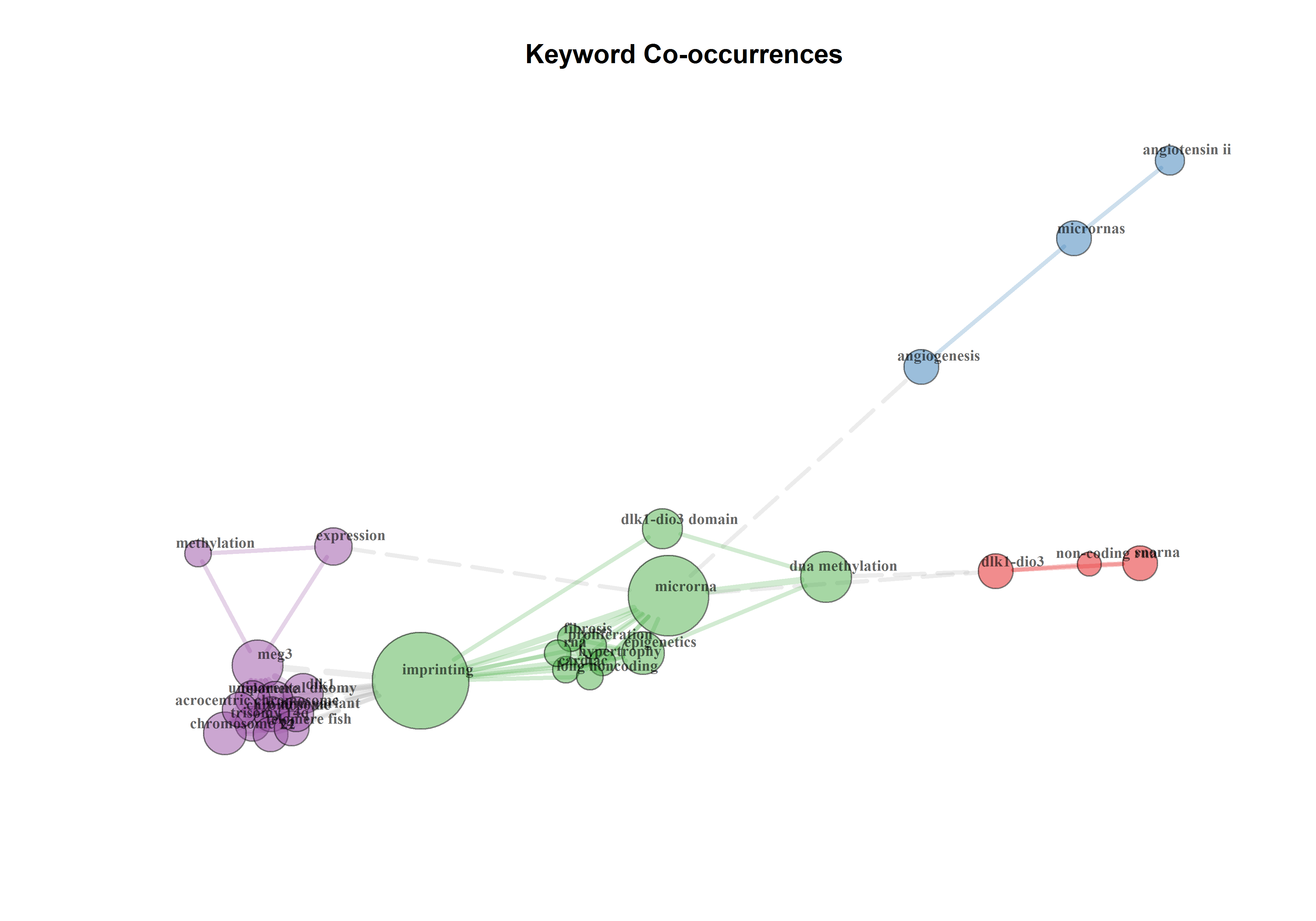
Genes and diseases analysis
Keywords are quite uninforamtive. I find that a better option is to use gene names and diseases identified by the NCBI Deep learning algorythm pubtator.
Pubtator query
Pubator returns all identifiers merged from a PMID list. Here we want this information for each articles so we need to do this iteratively.
# pubtator_o <- list()
# for (i in 1:length(M$PM)) {
#   pubtator_o[[i]] <- pubtator_function(M$PM[i])
#   if (isInteger(i/100)) {
#     print(i)
#   }
# }
# export(pubtator_o, "data_litterature_14q32/14q32_OR_DLK1-DIO3_AND_heartORcardio_pubtator.rds")

pubtator_o <- import("data_litterature_14q32/14q32_OR_DLK1-DIO3_AND_heartORcardio_pubtator.rds")
Network analysis of genes
Text needs to be reformated to be processed with the bibliometrix package
do <- as.data.frame(do.call(rbind, lapply(pubtator_o, as.character)), stringsAsFactors = F)
colnames(do) <- names(pubtator_o[[1]])
do <- do %>% replace(.=="NULL", NA)
do <- do[do$PMID != " No Data ",]

do <- apply(do,2,function(x) gsub("c[(]", "", x))
do <- apply(do,2,function(x) gsub("[)]", "", x))
do <- as.data.frame(apply(do, 2,function(x) gsub("\"", "", x)), stringsAsFactors = F)
do <- as.data.frame(apply(do, 2,function(x) gsub(">[0-9]+","", x)), stringsAsFactors = F)
do <- as.data.frame(apply(do, 2,function(x) gsub(">MESH:[A-Z][0-9]+","", x)), stringsAsFactors = F)
do <- as.data.frame(apply(do, 2,function(x) gsub(">-","", x)), stringsAsFactors = F)
do <- as.data.frame(apply(do, 2,function(x) gsub(",",";", x)), stringsAsFactors = F)
Now we can replace Keywords with the columns for Genes and/or Diseases from Pubtator
M2 <- M # new df to replace ID
df <- merge(M, do, by.x="PM", by.y = "PMID", all.x = T)


change_ID <- function(new_ID, DF) {
  # remove duplicated gene names (some are capitalized and others not)
  DF$ID <- new_ID
  DF$ID <- gsub("NA","",DF$ID)
  t <- split(toupper(DF$ID), seq(length(DF$ID)))
  t <- lapply(t, function(x) unique(str_trim(strsplit(x, ";")[[1]])))
  t <- lapply(t, function(x) paste(x, collapse = ";"))
  DF$ID <- unlist(t)
  DF$ID <- gsub("NULL","",DF$ID)
  return(DF)
}

new_ID <- paste0(df$Genes) # replacing ID with genes from Pubtator
M2 <- change_ID(new_ID,M2)

##### These other functions may also be helpful.
# summary(results2)
# CS <- conceptualStructure(M2,field="ID", method="CA", minDegree=4, clust=5, stemming=FALSE, labelsize=10, documents=10)

# rio::export(M2, "data_litterature_14q32/14q32_lit.xlsx") # to import in shiny
# biblioshiny()
NetMatrix <- biblioNetwork(M2, analysis = "co-occurrences", network = "keywords", sep = ";")
net=networkPlot(NetMatrix, normalize="association", weighted=T, n = 30, Title = "Keyword Cooccurrences", type = "auto", size=T,edgesize = 5)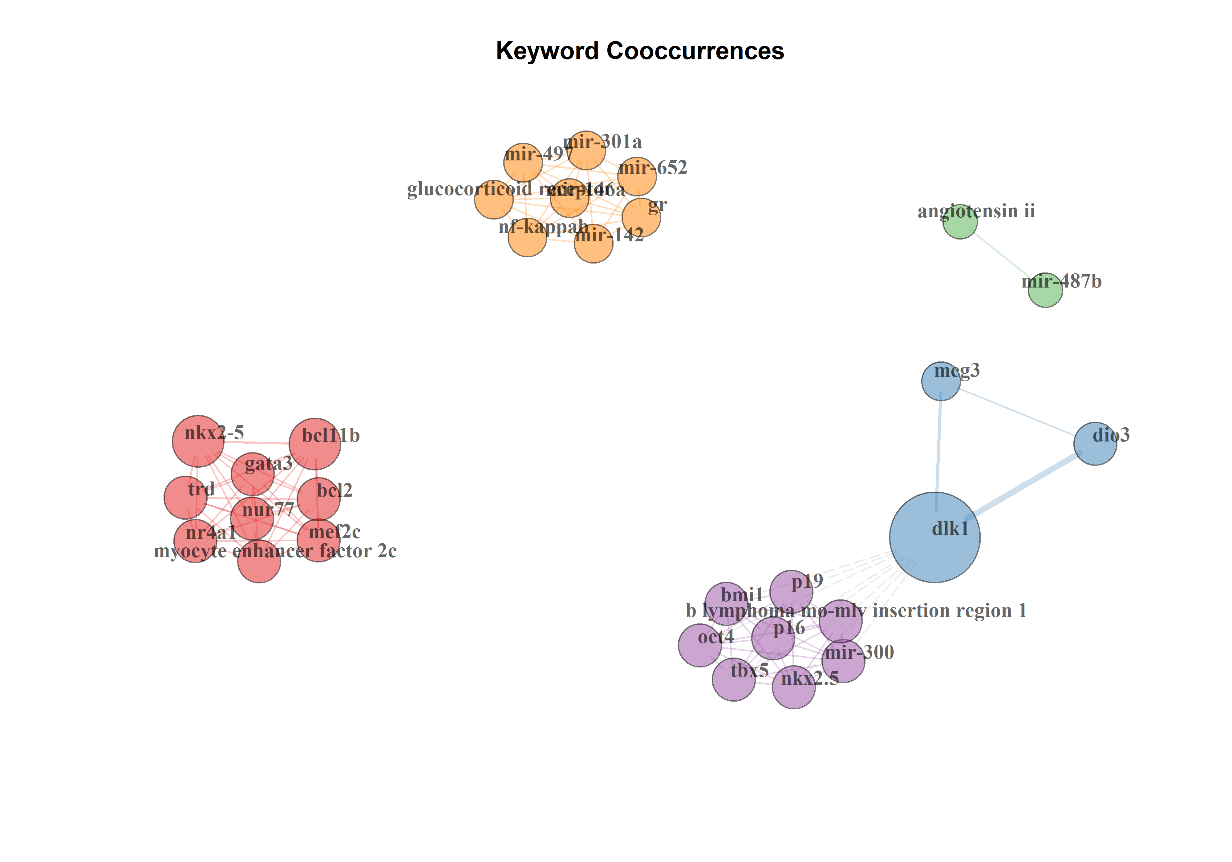
Variation of investigated genes over time
ID_evol_p <- function(DF, top_n_ID) {
  KWG_df <- KeywordGrowth(DF, Tag = "ID", sep = ";", top = top_n_ID, cdf = TRUE)
  m <- melt(KWG_df,  measure.vars = c(colnames(KWG_df)[2:(top_n_ID+1)]))
  m <- m %>% mutate(label = if_else(Year == max(Year), as.character(variable), NA_character_))

  labelInfo <-
    split(m, m$variable) %>%
    lapply(function(t) {
      data.frame(
        predAtMax = loess(value ~ Year, data = t) %>%
          predict(newdata = data.frame(Year = max(t$Year)))
        , max = max(t$Year)
      )}) %>%
    bind_rows

  labelInfo$label = levels(factor(m$variable))

  p <- ggplot(m, aes(x=Year, y=value, colour=variable))+
    geom_smooth(se=F) +
    geom_label_repel(data = labelInfo,
                     aes(x = max, y = predAtMax,
                         label = label,
                         color = label),
                     size = 3,
                     nudge_x = 5) +
    theme_minimal() +
    theme(legend.position = "none")+
    xlim(min(m$Year), 10+max(m$Year))+
    ylab("Cumulative frequency")
  return(p)
}

ID_evol_p(M2,30)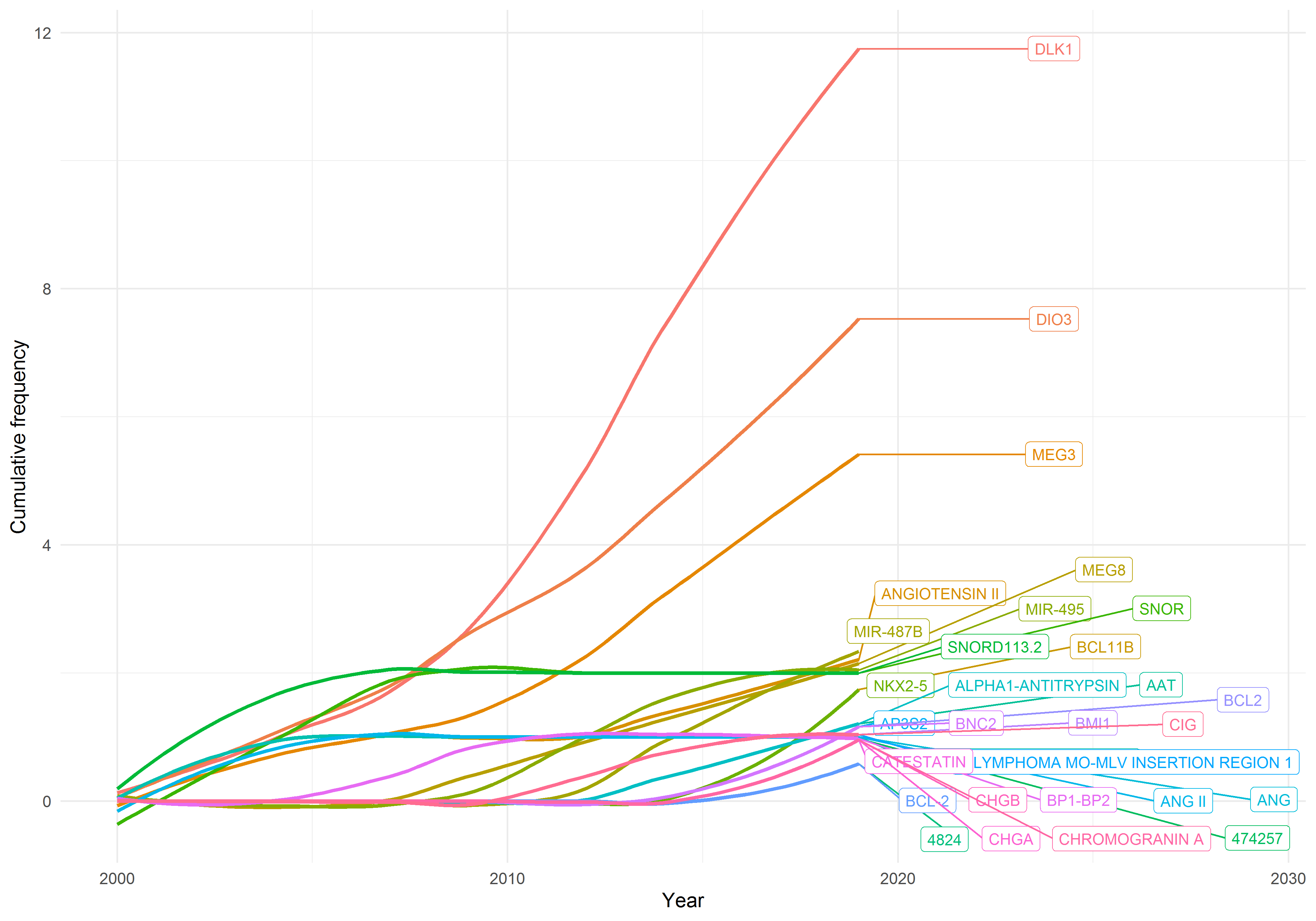
Network analysis of diseases
new_ID <- paste0(df$Diseases) # replacing ID with genes from Pubtator
M2 <- change_ID(new_ID,M2)
NetMatrix <- biblioNetwork(M2, analysis = "co-occurrences", network = "keywords", sep = ";")
net=networkPlot(NetMatrix, normalize="association", weighted=T, n = 50, Title = "Keyword Cooccurrences", type = "auto", size=T,edgesize = 5,labelsize=0.7)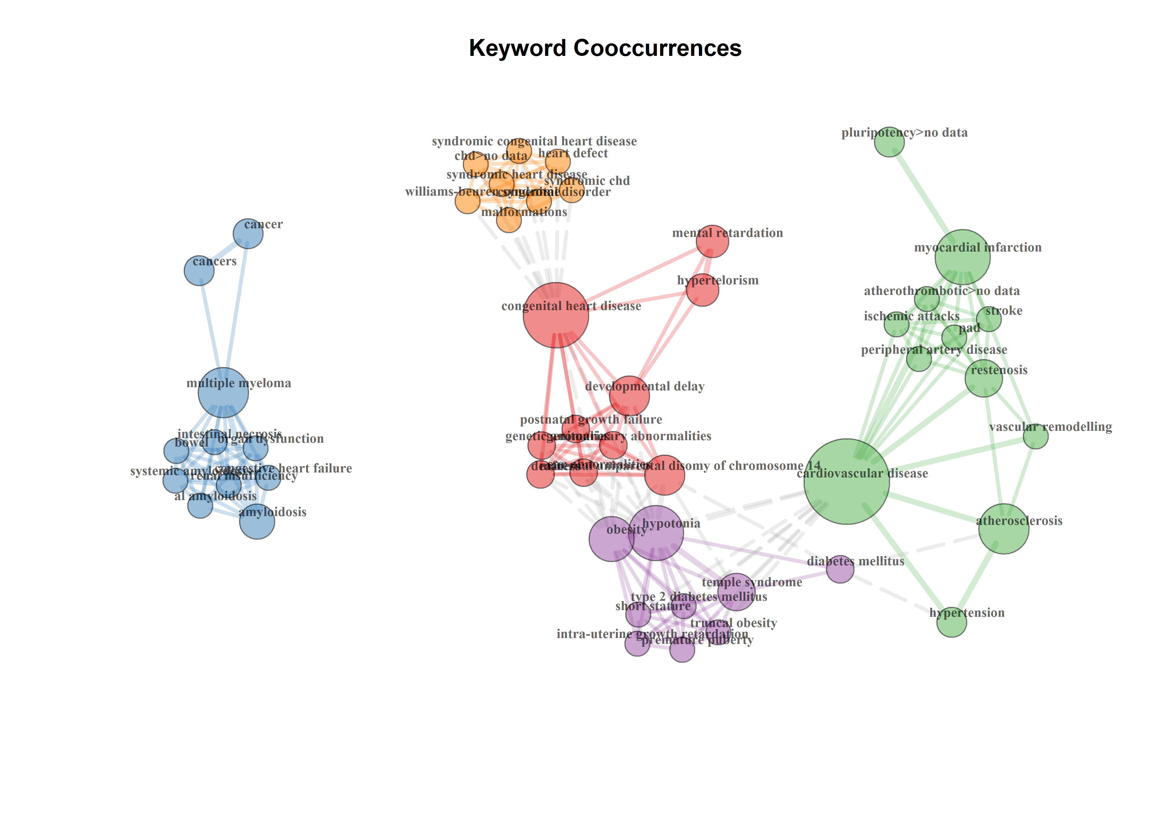
Variation of investigated diseases over time
ID_evol_p(M2,30)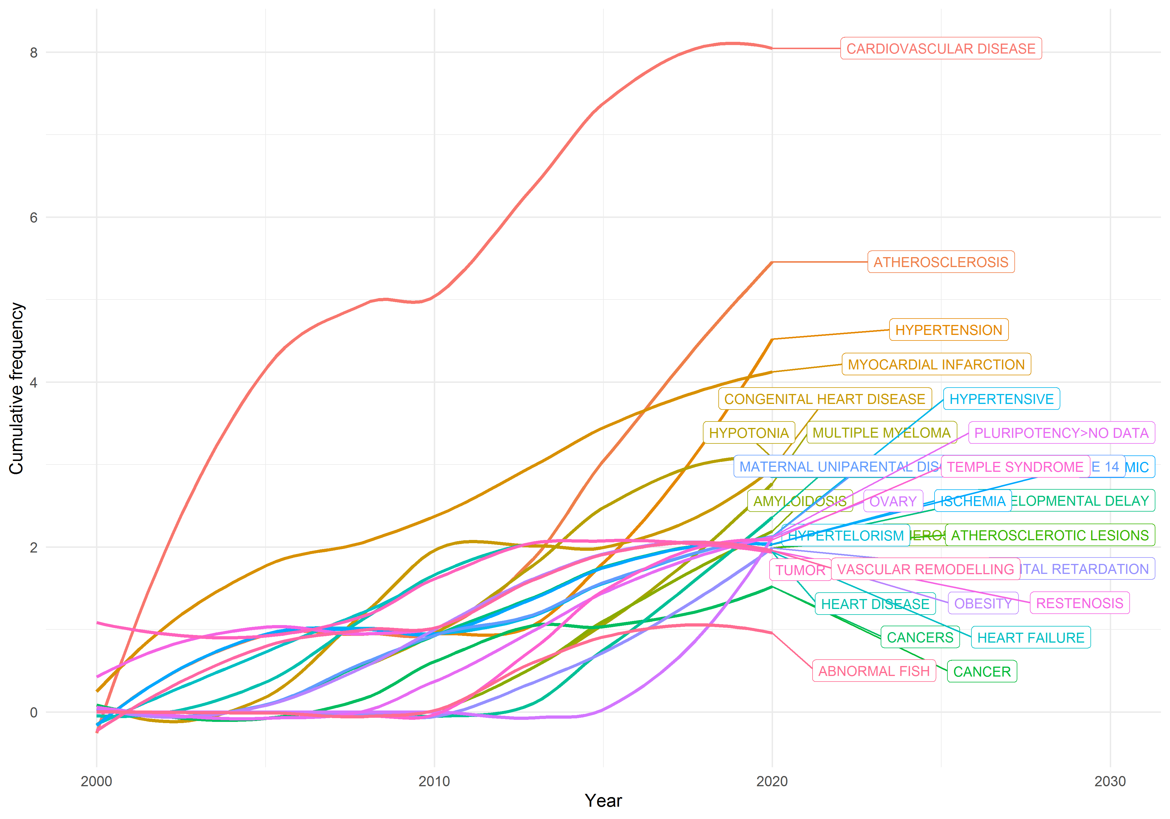
Combined genes and diseases network
new_ID <- paste0(df$Genes, ";",df$Diseases)
M2 <- change_ID(new_ID,M2)
results2 <- biblioAnalysis(M2, sep = ";")
# summary(results2)
# rio::export(M2, "data_litterature_14q32/14q32_lit.xlsx")
NetMatrix <- biblioNetwork(M2, analysis = "co-occurrences", network = "keywords", sep = ";")
net=networkPlot(NetMatrix, normalize="association", weighted=T, n = 50, Title = "Keyword Cooccurrences", type = "auto", size=T,edgesize = 5,labelsize=0.7)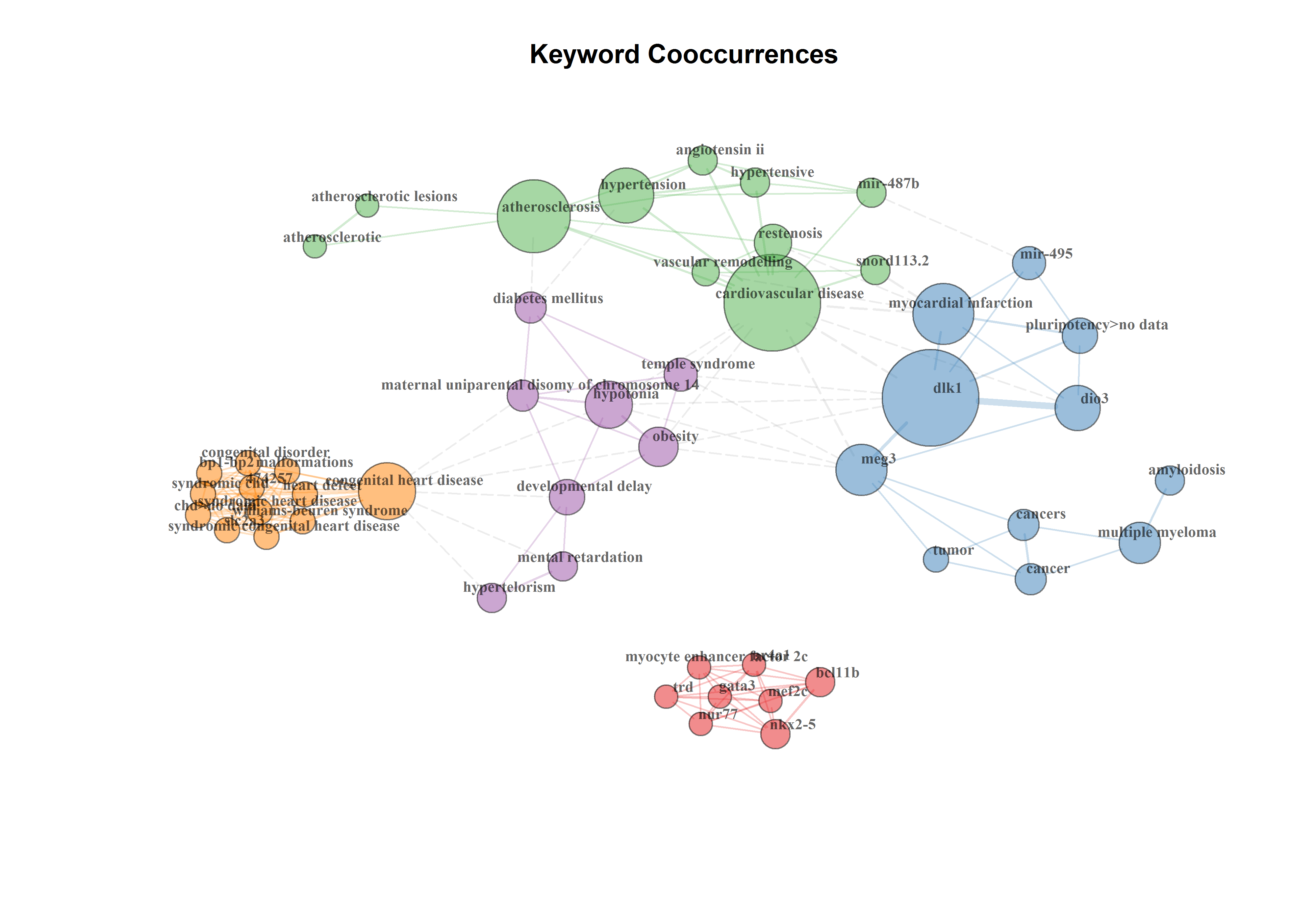
library("wordcloud")
set.seed(1234)
d <- as.data.frame(results2$ID)
wordcloud(words = d$Tab, freq = d$Freq, min.freq = 2,
          max.words=200, random.order=FALSE, rot.per=0.35,
          colors=brewer.pal(8, "Dark2"))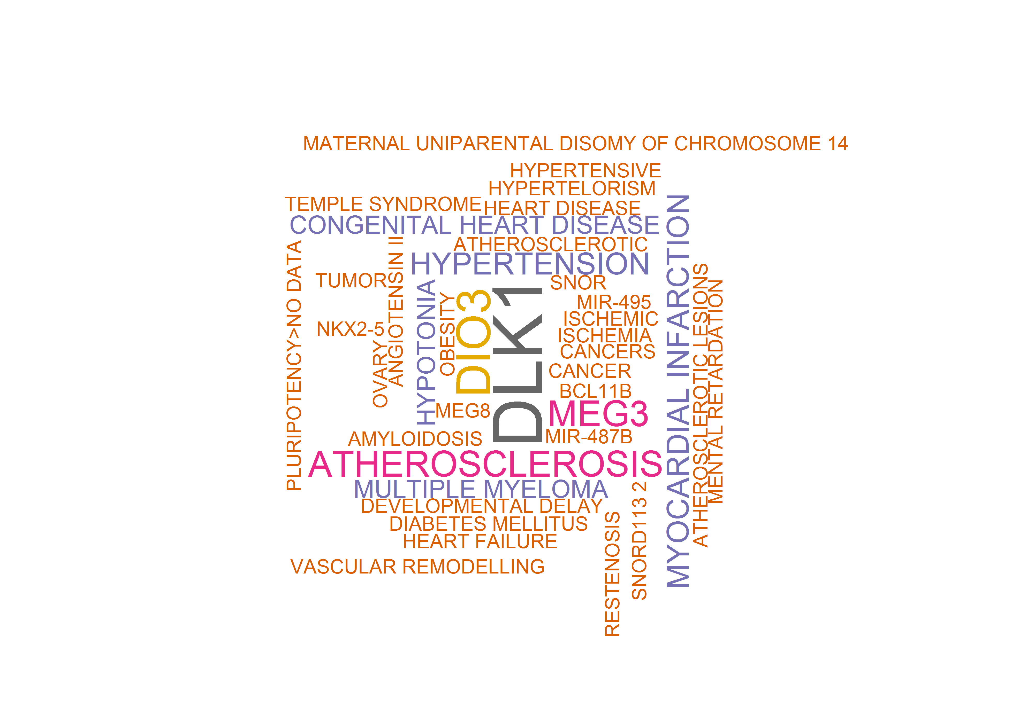
Best journal in topic
- number of citation per paper per year
- compare to their impact factor
sources <- data.frame(sources = M2$SO , TCperYear = results2$TCperYear)
sources <- sources %>% group_by(sources) %>% summarise(TCpY = sum(TCperYear))
sources$n_aticles <- M2 %>% group_by(SO) %>% count() %>% pull(n)
sources$TCpYpA <- sources$TCpY/sources$n_aticles


impact <- get_impactfactor(journals=sources$sources, max.distance = 0.1)
sources <- merge(sources, impact, by.x="sources", by.y = "Journal", all.x = T)
sources <- sources[!duplicated(sources$sources),]
top_J <- head(sources[order(sources$TCpYpA, decreasing = T),], 15)
ggplot(top_J, aes(y=reorder(sources,TCpYpA),x=TCpYpA))+
geom_bar(stat = "identity") +
theme_minimal()+
theme(legend.position = "none")+
xlab("Citations/(Years*Articles)")+
ylab("Journal")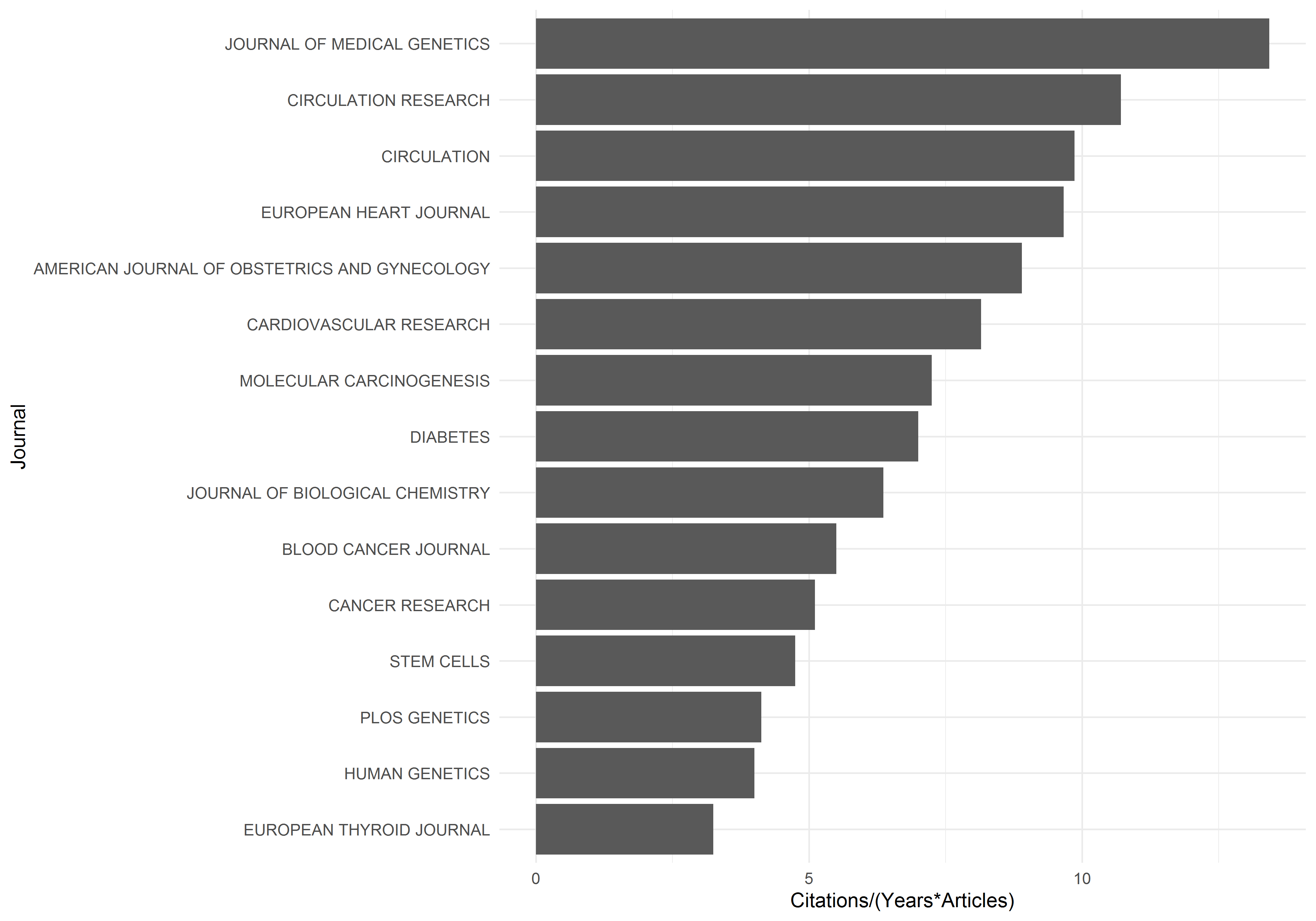
ggplot(top_J, aes(x = ImpactFactor, y=TCpYpA, label=sources, colour=sources))+
  geom_point() +
  geom_label_repel(size = 2.3)+
  scale_y_log10() +
  scale_x_log10() +
  theme_minimal() +
  theme(legend.position = "none") +
  ylab("Citations/(Years*Articles)")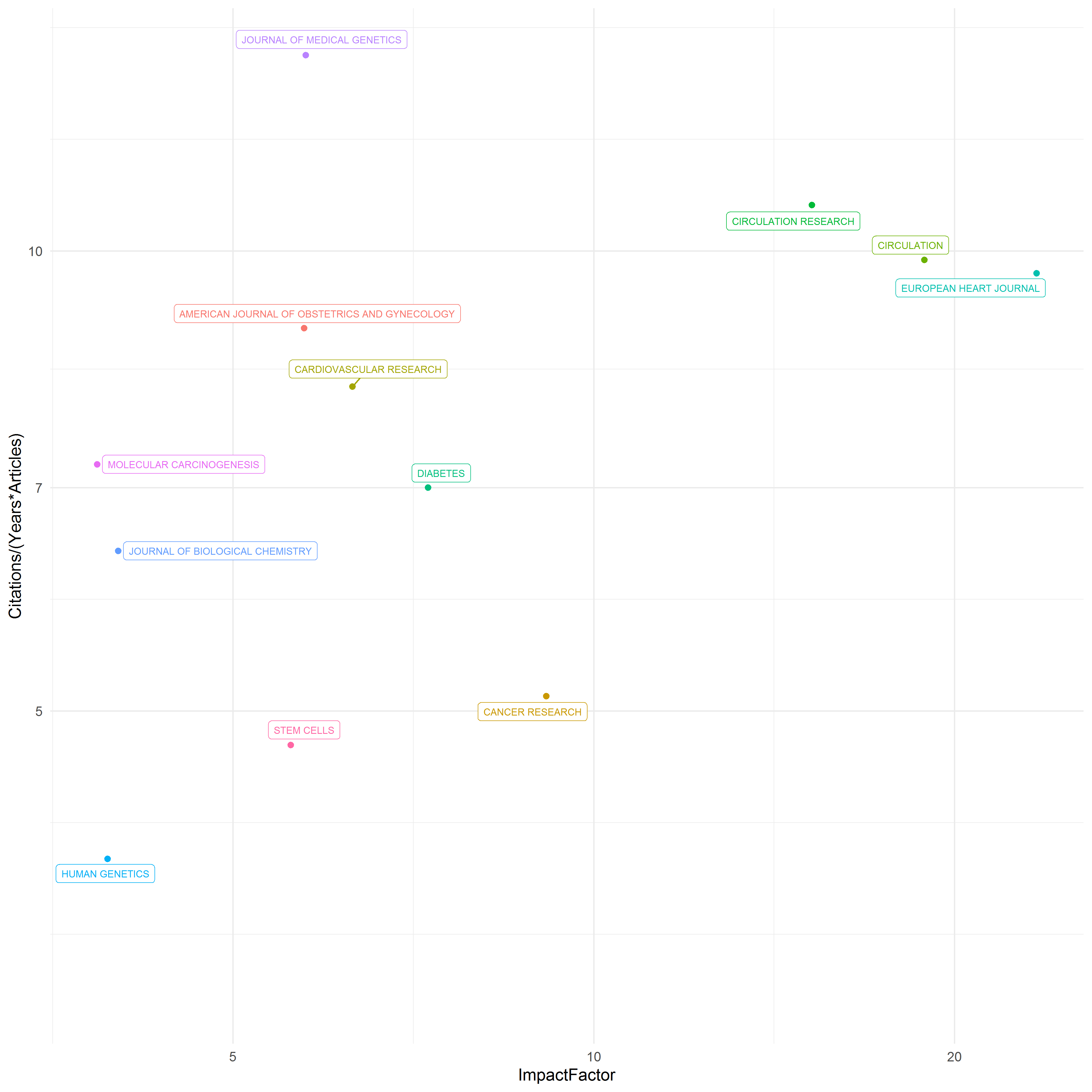
Large queries analyses
##### Function to get citation count from PMID
##### (modified from RISmed package to avoid errors from multiple queries)
f <- function(id){

  base <- "https://eutils.ncbi.nlm.nih.gov/entrez/eutils/elink.fcgi?retmode=xml&dbfrom=pubmed&id=ID&cmd=neighbor"
  base <- sub("ID", id, base)

  the_url <- url(description = base)
  on.exit(close(the_url))

  lines <- readLines(the_url)

  citedstart <- grep("pubmed_pubmed_citedin", lines)

  if(length(citedstart) == 0){
    return(0)
  }
  else{
    citedend <- grep("pubmed_pubmed", lines)
    citedend <- min(citedend[citedend > citedstart])

    tags <- grep("<Id>", lines)
    tags <- tags[tags > citedstart & tags < citedend]

    if(any(tags)){
      hits <- sub("(.*<ID>)([0-9]+)(.*)","\\2",lines[tags])
      hits <- unique(hits)
      length(hits[hits != id])
    }
    else{
      0
    }
  }
}

# get
library(pubmedR)
query <- "atrial fibrillation[Title/Abstract]"
res <- pmQueryTotalCount(query = query, api_key = NULL)
D <- pmApiRequest(query = query, limit = 100000, api_key = NULL)
M <- pmApi2df(D)


library(ttutils)
v <- c()
for (i in 1:length(M$PMID)) {
  v <- c(v,f(M$PMID[i])) # get citations 1 by one with sleep to avoid errors
  Sys.sleep(0.3)
  if (isInteger(i/100)) { # follow the long process
    print(i)
  }
}

# get Genes, Diseases, Mutations, Chemicals, Species from pubtator
library(pubmed.mineR)
pubtator_o <- list()
for (i in 1:length(M$PMID[1:100])) {
  pubtator_o[[i]] <- pubtator_function(M$PMID[i])
  if (isInteger(i/100)) {
    print(i)
  }
}sessionInfo()## R version 3.6.1 (2019-07-05)
## Platform: x86_64-w64-mingw32/x64 (64-bit)
## Running under: Windows 7 x64 (build 7601) Service Pack 1
##
## Matrix products: default
##
## locale:
## [1] LC_COLLATE=French_Canada.1252 LC_CTYPE=French_Canada.1252
## [3] LC_MONETARY=French_Canada.1252 LC_NUMERIC=C
## [5] LC_TIME=French_Canada.1252
##
## attached base packages:
## [1] stats graphics grDevices utils datasets methods base
##
## other attached packages:
## [1] wordcloud_2.6 RColorBrewer_1.1-2 reshape2_1.4.4
## [4] scholar_0.1.7 ggrepel_0.8.2 forcats_0.5.0
## [7] stringr_1.4.0 dplyr_1.0.0 purrr_0.3.4
## [10] readr_1.3.1 tidyr_1.0.2 tibble_3.0.0
## [13] ggplot2_3.3.1 tidyverse_1.3.0 ttutils_1.0-1
## [16] rio_0.5.16 pubmed.mineR_1.0.16 bibliometrix_3.0.2
##
## loaded via a namespace (and not attached):
## [1] colorspace_1.4-1 ellipsis_0.3.1 R2HTML_2.3.2
## [4] fs_1.4.1 rstudioapi_0.11 dimensionsR_0.0.1
## [7] farver_2.0.3 graphlayouts_0.7.0 rscopus_0.6.6
## [10] SnowballC_0.7.0 DT_0.13 fansi_0.4.1
## [13] lubridate_1.7.8 xml2_1.3.0 splines_3.6.1
## [16] codetools_0.2-16 R.methodsS3_1.8.0 leaps_3.1
## [19] knitr_1.28 shinythemes_1.1.2 polyclip_1.10-0
## [22] jsonlite_1.6.1 broom_0.5.6 cluster_2.1.0
## [25] dbplyr_1.4.4 R.oo_1.23.0 ggforce_0.3.1
## [28] shiny_1.4.0.2 rentrez_1.2.2 compiler_3.6.1
## [31] httr_1.4.1 backports_1.1.6 assertthat_0.2.1
## [34] Matrix_1.2-18 fastmap_1.0.1 cli_2.0.2
## [37] later_1.0.0 tweenr_1.0.1 htmltools_0.4.0
## [40] tools_3.6.1 igraph_1.2.5 gtable_0.3.0
## [43] glue_1.4.1 FactoMineR_2.3 Rcpp_1.0.4.6
## [46] cellranger_1.1.0 vctrs_0.3.0 nlme_3.1-147
## [49] blogdown_0.20 ggraph_2.0.2 xfun_0.14
## [52] networkD3_0.4 openxlsx_4.1.4 rvest_0.3.5
## [55] mime_0.9 lifecycle_0.2.0 pacman_0.5.1
## [58] shinycssloaders_0.3 XML_3.99-0.3 stringdist_0.9.6
## [61] factoextra_1.0.7 MASS_7.3-51.5 scales_1.1.1
## [64] tidygraph_1.1.2 hms_0.5.3 promises_1.1.0
## [67] parallel_3.6.1 yaml_2.2.1 curl_4.3
## [70] gridExtra_2.3 stringi_1.4.6 boot_1.3-25
## [73] zip_2.0.4 rlang_0.4.6 pkgconfig_2.0.3
## [76] bitops_1.0-6 evaluate_0.14 lattice_0.20-40
## [79] labeling_0.3 htmlwidgets_1.5.1 tidyselect_1.1.0
## [82] plyr_1.8.6 magrittr_1.5 bookdown_0.19
## [85] R6_2.4.1 generics_0.0.2 DBI_1.1.0
## [88] mgcv_1.8-31 withr_2.2.0 pillar_1.4.4
## [91] haven_2.2.0 foreign_0.8-76 scatterplot3d_0.3-41
## [94] RCurl_1.98-1.1 modelr_0.1.8 crayon_1.3.4
## [97] rmarkdown_2.2 viridis_0.5.1 grid_3.6.1
## [100] readxl_1.3.1 data.table_1.12.8 blob_1.2.1
## [103] reprex_0.3.0 digest_0.6.25 flashClust_1.01-2
## [106] R.cache_0.14.0 xtable_1.8-4 httpuv_1.5.2
## [109] R.utils_2.9.2 munsell_0.5.0 viridisLite_0.3.0
## [112] pubmedR_0.0.3
Francis Leblanc
PhD student in Bioinformatics
I am passionate about leveraging new omic technologies to enhance human healthspan.